Tuesday, December 30, 2008

Pleural versus Peritoneal Mesotheliomas

As discussed previously, it is possible to create an age distribution for the occurrence of every neoplasm listed in the SEER (NCI's Surveillance Epidemiology and End Results) public data set. It is also possible to determine the rate of occurrences, by age, normalized against population data. The numeric distributions and their graphic representations for over 700 types of neoplasms included in the SEER data, is available at:

http://www.julesberman.info/seerdist.pdf

With this data, it is possible to review the graphic distributions and to find trends or anomalies of biologic importance.

For example, consider the occurrences of mesothelioma, by age, and by site, comparing mesotheliomas of the pleura and of the peritoneum.


Crude occurrences of pleural mesothelioma, by age
Crude - 0 0 0 3 4 9 27 45 88 184 310 495 664 885 1066 1075 759 412


Normalized rate of pleural mesotheliomas
Normalized - 0 0 0 1 2 4 13 19 39 92 178 370 617 927 1202 1451 1540 975


Crude occurrences of peritoneal mesothelioma, by age
Crude - 0 0 0 3 4 11 12 21 30 40 48 83 110 103 107 75 44 27


Normalized rate of peritoneal mesotheliomas
Normalized - 0 0 0 1 2 5 5 9 13 20 27 62 102 107 120 101 89 63

From the numbers, it is clear that pleural mesothelioma occurs much more frequently than peritoneal mesothelioma.

In addition, there seems to be about a ten year difference in the peak age of occurrence of pleural and peritoneal mesotheliomas. Peritoneal mesotheliomas seem to occur in a slightly younger age group.

How can we determine whether this apparent difference in the age distributions of pleural and peritoneal mesotheliomas is, in fact, significant?

A short Perl script calls an external statistics module that accepts the normalized age distributions of pleural and peritoneal mesotheliomas and applies the F and Student t tests. (Note: you must install the Statistics::TTest module to run the script)

#!/usr/bin/perl
use Statistics::PointEstimation;
use Statistics::TTest;
open(STDOUT, ">tftest.txt");
my @r1=qw(0 0 0 1 2 4 13 19 39 92 178 370 617 927 1202 1451 1540 975);
my @r2=qw(0 0 0 1 2 5 5 9 13 20 27 62 102 107 120 101 89 63);
my $ttest = new Statistics::TTest;
$ttest->set_significance(98);
$ttest->load_data(\@r1,\@r2);
$ttest->output_t_test();
$ttest->print_t_test(); #list out t-test related data
exit;


The output is shown:

Click on the image to see a larger format.

The Perl script produces an F-test and t-test statistic for the distribution of normalized mesothelioma rates, for pleural and peritoneal sites, by age.

We can be confident, at a 98% confidence level, that there is a difference in the population that develops pleural mesothelioma, compared with the population that develops peritoneal mesothelioma.

What can account for this difference? Assuming no statistical error (i.e., falsely rejecting the null hypothesis), I see four possibilities.

1. Multiple diseases in one name
(i.e. peritoneal mesothelioma may be a biologically distinct neoplasm, different from pleural mesothelioma).

2. Multiple environmental causes
(i.e. the causes of pleural mesothelioma are different from the causes of peritoneal mesothelioma, resulting in a different age distribution of these tumors).

3. Multiple genetic causes with different latencies
(i.e., gene variants that predispose pleural mesothelioma may be different from gene variants that predispose peritoneal mesothelioma, accounting for different latency periods and differences in the age distribution of tumors)

4. Faulty or insufficient data
(i.e. the differences are due to faulty data)

5. Combinations of 1,2,3, and 4

If anyone reading this blog can think of any other explanation(s), please comment.

Other web pages related to this topic are:

http://www.julesberman.info/seerdist.pdf

http://www.julesberman.info/seer2.htm

http://www.julesberman.info/cdc_ch.pdf

-© 2008 Jules Berman

As with all of my scripts, lists, web sites, and blog entries, the following disclaimer applies. This material is provided by its creator, Jules J. Berman, "as is", without warranty of any kind, expressed or implied, including but not limited to the warranties of merchantability, fitness for a particular purpose and noninfringement. In no event shall the author or copyright holder be liable for any claim, damages or other liability, whether in an action of contract, tort or otherwise, arising from, out of or in connection with the material or the use or other dealings.

key words: pleura, peritoneum, abdominal mesothelioma, subtype, neoplasms, neoplasms, carcinogenesis, epidemiology
In June, 2014, my book, entitled Rare Diseases and Orphan Drugs: Keys to Understanding and Treating the Common Diseases was published by Elsevier. The book builds the argument that our best chance of curing the common diseases will come from studying and curing the rare diseases.


I urge you to read more about my book. There's a generous preview of the book at the Google Books site.

Why I write scripts in Perl, Ruby and Python

Readers of this blog know that I often include equivalent scripts in Perl, Ruby and Python, for the biomedical informatics projects that I post.

It must be tedious to encounter a blog that devotes long stretches of space to scripts written in three different languages. I can imagine the groans coming from non-programmers when they see a long post full of code, while all they're interested in is the biomedical problem described in the first paragraph of the post.

I have reasons for including these scripts:

1. I want to reach all of the people who are interested in the biomedical problems discussed in my posts. Most of these problems are solved with informatics techniques. The techniques often involve a little bit of programming knowledge. Most biomedical programming is done with Perl, Ruby or Python. These are free, open source and cross-platform languages with active user communities and with abundant instructional material on the internet. If I want to attract the maximum number of readers, I've got to include solutions in all three languages.

2. I want to show readers that powerful scripts, that solve important biomedical problems, can be written in a few lines of code, regardless of the language used. Perl, Ruby and Python can all be used to write equivalent programs. For length, clarity, and speed of execution, there really isn't much difference among the major scripting languages. Biomedical scripts tend to use a few favorite commands (open a file, parse the file line by line, extract something from the lines of the file, do some sort of transformation on the extracted data, write the results to another file). These commands can be learned in a few hours.

3. I want to emphasize in all of my blogs that the difficult part in any informatics project is developing your question (i.e., asking a smart, important, and solvable question), and understanding the substance and limitations of the available data sources. Writing scripts is the easiest and most enjoyable part of the exercise.

- © 2008 Jules J. Berman
Science is not a collection of facts. Science is what facts teach us; what we can learn about our universe, and ourselves, by deductive thinking. From observations of the night sky, made without the aid of telescopes, we can deduce that the universe is expanding, that the universe is not infinitely old, and why black holes exist. Without resorting to experimentation or mathematical analysis, we can deduce that gravity is a curvature in space-time, that the particles that compose light have no mass, that there is a theoretical limit to the number of different elements in the universe, and that the earth is billions of years old. Likewise, simple observations on animals tell us much about the migration of continents, the evolutionary relationships among classes of animals, why the nuclei of cells contain our genetic material, why certain animals are long-lived, why the gestation period of humans is 9 months, and why some diseases are rare and other diseases are common. In “Armchair Science”, the reader is confronted with 129 scientific mysteries, in cosmology, particle physics, chemistry, biology, and medicine. Beginning with simple observations, step-by-step analyses guide the reader toward solutions that are sometimes startling, and always entertaining. “Armchair Science” is written for general readers who are curious about science, and who want to sharpen their deductive skills.

Monday, December 29, 2008

Perl, Ruby and Python scripts for CDC public use mortality file parsing

I have been interested in knowing whether sickle cell incidence is decreasing in the U.S. population. Despite Pubmed and web searches, I have not been able to find a single data source on the subject. In a prior post, I referred to one of my Perl scripts that
parsed through CDC public use records (about 5 Gigabytes of raw data). The results seemed to suggest that the incidence of sickle cell anemia in the U.S. may be increasing.

For those interested, here are Perl, Ruby and Python versions of the script that parses through the CDC public use mortality files for the years 1996, 1999, 2002, and 2004, to produce the number of occurrences and the rates for sickle cell disease cases, from death certificate data, for those years.

Please refer to the prior post for discussion of the data.

Please refer to my document describing uses for the CDC public use mortality files for general instructions on acquiring and analyzing the de-identified U.S. death certificate data.

#!/usr/local/bin/perl
@filearray = qw(mort96us.dat mort99us.dat mort02us.dat mort04us.dat);
foreach $file (@filearray)
{
open (ICD, $file);
$line = " ";
$popcount = 0;
$counter = 0;
while ($line ne "")
{
$line = <ICD>;
$codesection = substr($line,448,140) if ($file eq $filearray[0]);
$codesection = substr($line,161,140) if ($file eq $filearray[1]);
$codesection = substr($line,162,140) if ($file eq $filearray[2]);
$codesection = substr($line,164,140) if ($file eq $filearray[3]);
$popcount++;
if ($codesection =~ /D57/i)
{
$counter++;
}
}
close ICD;
$rate = $counter / $popcount;
$rate = substr((100000 * $rate),0,5);
print "\n\nRecords listing sickle cell is $counter in $file file";
print "\nSickle cell rate per 100,000 records is $rate in $file file";
}
exit;

#!/usr/local/bin/ruby
filearray = Array.new
filearray = "mort96us.dat mort99us.dat mort02us.dat mort04us.dat".split
filearray.each do
|file|
text = File.open(file, "r")
counter = 0; popcount = 0;
text.each_line do
|line|
codesection = line[448,140] if (file == filearray.fetch(0))
codesection = line[161,140] if (file == filearray.fetch(1))
codesection = line[162,140] if (file == filearray.fetch(2))
codesection = line[164,140] if (file == filearray.fetch(3))
popcount = popcount +1
counter = (counter + 1) if (codesection =~ /D57/i)
end
text.close
rate = ((counter.to_f / popcount.to_f) * 100000).to_s[0,5]
puts "\nRecords listing sickle cell is #{counter} in #{file} file"
puts "Sickle cell rate per 100,000 records is #{rate} in #{file} file"
end
exit

#!/usr/local/bin/python
import re
sickle_match = re.compile('D57')
lst = ("mort96us.dat","mort99us.dat","mort02us.dat","mort04us.dat")
for file in lst:
intext = open(file, "r")
popcount = 0
counter = 0
codesection = ""
for line in intext:
if file == lst[0]:
codesection = line[448:588]
if file == lst[1]:
codesection = line[161:301]
if file == lst[2]:
codesection = line[162:302]
if file == lst[3]:
codesection = line[164:304]
popcount = popcount + 1
p = sickle_match.search(codesection)
if p:
counter = counter + 1
intext.close
rate = float(counter) / float(popcount) * 100000
rate = str(rate)
rate = rate[0:5]
print ('\n\nRecords listing sickle cell is ')
print (str(counter) + ' in ' + file + ' file')
print ('\nSickle cell rate per 100,000 records is ')
print(str(rate) + ' in ' + file + ' file')
exit

© 2008 Jules Berman

As with all of my scripts, lists, web sites, and blog entries, the following disclaimer applies. This material is provided by its creator, Jules J. Berman, "as is", without warranty of any kind, expressed or implied, including but not limited to the warranties of merchantability, fitness for a particular purpose and noninfringement. In no event shall the author or copyright holder be liable for any claim, damages or other liability, whether in an action of contract, tort or otherwise, arising from, out of or in connection with the material or the use or other dealings.

In June, 2014, my book, entitled Rare Diseases and Orphan Drugs: Keys to Understanding and Treating the Common Diseases was published by Elsevier. The book builds the argument that our best chance of curing the common diseases will come from studying and curing the rare diseases.


I urge you to read more about my book. There's a generous preview of the book at the Google Books site. If you like the book, please request your librarian to purchase a copy of this book for your library or reading room.

tags: common disease, orphan disease, orphan drugs, rare disease, disease genetics, sickle cell anemia, genetic counseling, public health, centers for disease control and prevention, international classification of diseases, cause of death, causes of death, epidemiology, Perl programming, Ruby programming, Python programming

Sunday, December 28, 2008

Updated cancer occurrence document now available

An updated version of my recently posted document, listing the age distributions for the occurrences of over 700 different human cancers, is now available at:

http://www.julesberman.info/seerdist.pdf.

The new version includes age occurrence rates, normalized against U.S. Census data.

In the next few weeks, I'll be posting on the clinical significance of some of the data contained in the document.

-Jules Berman
Science is not a collection of facts. Science is what facts teach us; what we can learn about our universe, and ourselves, by deductive thinking. From observations of the night sky, made without the aid of telescopes, we can deduce that the universe is expanding, that the universe is not infinitely old, and why black holes exist. Without resorting to experimentation or mathematical analysis, we can deduce that gravity is a curvature in space-time, that the particles that compose light have no mass, that there is a theoretical limit to the number of different elements in the universe, and that the earth is billions of years old. Likewise, simple observations on animals tell us much about the migration of continents, the evolutionary relationships among classes of animals, why the nuclei of cells contain our genetic material, why certain animals are long-lived, why the gestation period of humans is 9 months, and why some diseases are rare and other diseases are common. In “Armchair Science”, the reader is confronted with 129 scientific mysteries, in cosmology, particle physics, chemistry, biology, and medicine. Beginning with simple observations, step-by-step analyses guide the reader toward solutions that are sometimes startling, and always entertaining. “Armchair Science” is written for general readers who are curious about science, and who want to sharpen their deductive skills.

Saturday, December 27, 2008

Is the incidence of sickle cell disease rising?

In 1949, Linus Pauling and coworkers showed that sickle cell anemia is a disease produced by an inherited alteration in hemoglobin, producing a molecule that is separable from normal hemoglobin, by electrophoris. Electrophoresis is still used to distinguish sickle hemoglobin from normal hemoglobin.

In 1956, Vernon Ingram and J.A. Hunt sequenced the hemoglobin protein molecule (normal and sickle cell) and showed that the inherited alteration in sickle cell hemoglobin is due to a single amino acid substitution in the protein sequence.

Because sickle cell hemoglobin can be detected by a simple blood test, it was assumed, back in the 1950s, that new cases of this disease would be prevented through testing, followed by genetic counseling. Today, there are a number of private and public organizations that work to reduce the incidence of sickle cell disease.

I have been interested in knowing whether sickle cell incidence is decreasing in the U.S. population. Despite Pubmed and web searches, I have not been able to find a single data source on the subject.

I decided to investigate using the CDC (U.S. Centers for Disease Control and Prevention) mortality data sets. In a separate document, I've provided methods for acquiring and analyzing the CDC public use mortality files.

For the current study, I downloaded the mortality files for the years 1996, 1999, 2002, and 2004, all of which contain de-identified records listing multiple conditions, coded in ICD-10 (International Classification of Disease, version 10), for the underlying causes of death and other significant conditions, found on U.S. death certificates.

I parsed through every record (about 5 Gigabytes of raw data), and compiled the following results.

In 1996, U.S. cases with sickle cell disease in death certificates is 708
In 1996, U.S. rate of sickle cell disease in death certificates is 30.54 per 100,000

In 1999, U.S. cases with sickle cell disease in death certificates is 799
In 1999, U.S. rate of sickle cell disease in death certificates is 33.36 per 100,000

In 2002, U.S. cases with sickle cell disease in death certificates is 827
In 2002, U.S. rate of sickle cell disease in death certificates is 33.79 per 100,000

In 2004, U.S. cases with sickle cell disease in death certificates is 876
In 2004, U.S. rate of sickle cell disease in death certificates is 36.47 per 100,000

For all four years examined, there has been a steady, increasing trend in the number of death certificates listing sickle cell disease as a cause of death or a significant condition at the time of death. Likewise, the overall rate (per 100,000 certificates) has steadily increased in every sampled year, covering 1996 to 2004.

Does this mean that efforts to reduce the incidence of sickle cell disease have failed? No. Death certificate data is unreliable. Whether a doctor thinks of adding sickle cell disease as a medical condition, on the death certificate, may depend on a variety of factors (as discussed previously). However, when you're dealing with very large numbers, trends usually reflect reality.

The best data would be natality incidence rates, by year, measured between about 1960 and the present. However, I have not been able to find that kind of data, and the CDC mortality files may be the next-best option.

For those interested in conducting an independent analysis of the same data, here are the locations of the files that I downloaded by anonymous ftp from the CDC server (ftp.cdc.gov)

1999
/pub/Health_Statistics/NCHS/Datasets/mortality

2002, 2004
/pub/Health_Statistics/NCHS/Datasets/DVS/mortality

1996 data file that combines icd9 and 1cd10 data
/pub/Health_Statistics/NCHS/Datasets/Comparability/icd9_icd10

If anyone has access to more reliable data, or a different set of results, please add a comment to this blog.

- © 2008 Jules Berman

As with all of my scripts, lists, web sites, and blog entries, the following disclaimer applies. This material is provided by its creator, Jules J. Berman, "as is", without warranty of any kind, expressed or implied, including but not limited to the warranties of merchantability, fitness for a particular purpose and noninfringement. in no event shall the author or copyright holder be liable for any claim, damages or other liability, whether in an action of contract, tort or otherwise, arising from, out of or in connection with the material or the use or other dealings.

In June, 2014, my book, entitled Rare Diseases and Orphan Drugs: Keys to Understanding and Treating the Common Diseases was published by Elsevier. The book builds the argument that our best chance of curing the common diseases will come from studying and curing the rare diseases.


I urge you to read more about my book. There's a generous preview of the book at the Google Books site. If you like the book, please request your librarian to purchase a copy of this book for your library or reading room.

tags: common disease, orphan disease, orphan drugs, rare disease, disease genetics, cdc, epidemiology, sickle cell disease, sickle cell anemia, sickle cell anaemia, cdc, death certificate data, U.S. mortality tables, understanding death certificates, incidence of sickle cell disease, rate of sickle cell disease, cause of death, icd10, international classification of diseases

Friday, December 26, 2008

Cancer occurrence by age: distributions and schematics

I just posted, on my web site, a pdf document that compiles age occurrence data for the cancers included in the SEER public use data records (about 3.5 million records including over 700 kinds of cancers collected from 1973-2005).

For each cancer, I binned the number of occurrences of cancers into 5-year intervals, beginning with ages 0-5 and ending with ages 95 and above.

Specifically, each number following the name of the cancer is followed by 20 sequential intervals:

0-4,5-9,10-14,15-19,20-24....80-84,85-89,90-94,95+

In the document, a schematic representation follows each raw distribution.

The document provides pathologists with a guideline for the expected occurrences of cancers, by age. A good pathologist should be very careful when he/she assigns a diagnosis that does not "fit" the typical age profile of a cancer.

Epidemiologists may benefit by having a single source, indicating the likelihood of any types of specific cancer, in different age populations.

Researchers may, when reviewing all of the distributions at once, develop new questions and hypotheses that could not have been perceived through piecemeal observations.

The document is available at:

http://www.julesberman.info/seerdist.pdf

In the next few blogs, I'll provide excerpts from the document and explain how the document can be used for clinical and research purposes.

-© 2008 Jules Berman
My book, Principles of Big Data: Preparing, Sharing, and Analyzing Complex Information was published in 2013 by Morgan Kaufmann.


I urge you to explore my book. Google books has prepared a generous preview of the book contents.

tags: big data, metadata, data preparation, data analytics, data repurposing, datamining, data mining, epidemiology

Sunday, December 21, 2008

REPORT ON THE CDC MORTALITY DATA SETS

I've collected all of my recent blogs on the CDC (Centers for Disease Control and Prevention) mortality data sets and put them into a single pdf file for easy reading.

All of the included techniques, scripts, tools and data sets are open source. They include:

1. Methods for accessing publicly available de-identified records collected from death certficates

2. Methods to parse and analyze the CDC data sets

3. Methods for compiling an ICD10 (International Classification of Diseases version 10) data dictionary from publicly available sources

4. Methods for creating map mashups from publicly available data sets

5. Script examples (mostly in Perl) of the kinds of questions that can be answered with the public use data sets.

The report, intended for biomedical researchers who have some programming knowledge (preferably Perl, Ruby or Python), is about 3 Megabytes in length. It is available, at no cost, from:

http://www.julesberman.info/cdc_ch.pdf

-Jules J. Berman
My book, Principles of Big Data: Preparing, Sharing, and Analyzing Complex Information was published in 2013 by Morgan Kaufmann.


I urge you to explore my book. Google books has prepared a generous preview of the book contents.

tags: big data, metadata, data preparation, data analytics, data repurposing, datamining, data mining, epidemiology

Friday, December 19, 2008

CDC Mortality Data: 11th of 11 posts

This is the eleventh and final post in a series on the CDC mortality data sets. If you've been following this series, you've seen how easy it is to parse through a year's worth of de-identified death certificate data contained in one of the CDC public use mortality files.

We've been using the 1999 mortality file, which contains about 2.3 million records. Each record may list up to 20 diseases, representing the underlying and proximate causes of death and any significant additional conditions that the certifying doctor deems noteworthy.

How many diagnoses are typically listed on a death certificate? About 3. Many certificates list only a single condition

It's easy to rank the average number of conditions listed on the certificates, by state.

The lowest ranking state is AR (Arkansas), with an average of 2.442 conditions listed on each certificate. Next in line is Louisianna, with 2.47 conditions listed. Arizona follows with 2.501.

2.442 AR
2.479 LA
2.501 AZ
2.531 AL
2.554 MT
2.567 MA
2.579 NV
2.603 OK
2.603 VA
2.609 KY
2.621 IL
2.631 IN
2.632 WI
2.634 NM
2.649 OR
2.652 FL
2.663 MI
2.667 SD
2.678 MN
2.690 NJ
2.714 UT
2.768 AK
2.774 PA
2.781 MS
2.789 KS
2.795 MO
2.796 ID
2.800 WY
2.802 GA
2.824 SC
2.831 IA
2.855 ME
2.875 CO
2.875 TX
2.879 WA
2.880 NC
2.883 TN
2.903 DE
2.909 NH
2.921 NE
2.935 DC
2.949 NY
2.955 MD
2.956 CT
3.083 ND
3.102 WV
3.125 VT
3.138 OH
3.195 RI
3.316 HI
3.363 CA

The highest-ranking state is California, with 3.363 conditions listed on each certificate. Next to the top is Hawaii, with 3.316 conditions.

Here is the Perl script that produced the data.

#/usr/local/bin/perl
open (STATE, "cdc_states.txt"); #maps CDC state number
$line = " "; #to the state abbreviation
while ($line ne "")
{
$line = <STATE>;
$line =~ /^[0-9]{2}/;
$state_code = $&;
$line =~ / +([A-Z]{2}) *$/;
$state_abb = $1;
$statehash{$state_code} = $state_abb;
}
close STATE;
open (ICD, "Mort99us\.dat"); #the CDC mortality file
$line = " ";
while ($line ne "")
{
$line = <ICD>;
$codesection = substr($line,161,140);
$code = substr($line,20,2);
$state = $statehash{$code};
$state_total{$state}++;
$codesection =~ s/ +$//;
$eager = scalar(split(" ",$codesection));
$state_eager{$state} = $state_eager{$state} + $eager;
}
while ((my $key, my $value) = each(%state_total))
{
$goodness = substr(($state_eager{$key} / $value),0,5);
push(@list_array, "$goodness $key");
}
print join("\n", (sort(@list_array)));
exit;

What is a "lazy" death certificate? I would think that a lazy death certificate is one that contains the absolutely minimal number of conditions required to certify death (i.e., "1"). Let's rank the states by the fraction of death certificates, registered in the state, that contain only one listed condition for the cause of death (by tweaking the first Perl script).

0.323 AL
0.304 MT
0.303 AR
0.291 KY
0.290 IN
0.288 LA
0.285 MN
0.277 VA
0.274 WI
0.270 SD
0.267 MI
0.267 IL
0.258 PA
0.255 OK
0.255 MA
0.252 OR
0.249 NM
0.249 NJ
0.245 MO
0.244 AZ
0.242 ID
0.241 ME
0.241 FL
0.239 AK
0.238 UT
0.238 KS
0.234 WA
0.233 IA
0.229 DE
0.228 WY
0.225 SC
0.222 TN
0.222 CO
0.221 NC
0.220 TX
0.219 NV
0.217 DC
0.214 MS
0.214 MD
0.200 GA
0.199 NH
0.196 OH
0.192 WV
0.190 ND
0.185 NE
0.180 RI
0.177 VT
0.176 CT
0.171 HI
0.129 NY
0.119 CA

Alabama has the worst performance, with nearly one third of death certificates having only 1 listed condition. California, once more, has the best performance of all the states, with one condition reported in only about one tenth of certificates (i.e., about 90% of certificates have more than one condition reported).

Just about every death involves multiple underlying causes of death leading to a proximate cause of death. The number of conditions listed on a death certificate is, in most cases, a matter of personal effort on the part of the certifying doctor.

As we discussed in an earlier blog in this series, it can be quite difficult to produce an accurate death certificate. Nonetheless, much of what we know about human disease and the causes of human mortality come from examination of death certificates. Death certificates have profound importance to the family of the deceased. Doctors should be trained to provide complete and accurate entries for "causes of death" and "other significant conditions" on death certificates.

As I remind readers in almost every blog post, if you want to do your own creative data mining, you will need to learn a little about computer programming.

For Perl and Ruby programmers, methods and scripts for using a wide range of publicly available biomedical databases, are described in detail in my prior books:

Perl Programming for Medicine and Biology

Ruby Programming for Medicine and Biology

An overview of the many uses of biomedical information is available in my book,
Biomedical Informatics.

More information on cancer is available in my recently published book, Neoplasms: Principles of Development and Diversity.

© 2008 Jules Berman

As with all of my scripts, lists, web sites, and blog entries, the following disclaimer applies. This material is provided by its creator, Jules J. Berman, "as is", without warranty of any kind, expressed or implied, including but not limited to the warranties of merchantability, fitness for a particular purpose and noninfringement. in no event shall the author or copyright holder be liable for any claim, damages or other liability, whether in an action of contract, tort or otherwise, arising from, out of or in connection with the material or the use or other dealings.

In June, 2014, my book, entitled Rare Diseases and Orphan Drugs: Keys to Understanding and Treating the Common Diseases was published by Elsevier. The book builds the argument that our best chance of curing the common diseases will come from studying and curing the rare diseases.


I urge you to read more about my book. There's a generous preview of the book at the Google Books site. If you like the book, please request your librarian to purchase a copy of this book for your library or reading room.

Thursday, December 18, 2008

CDC Mortality Data: 10

This is the tenth in a series of posts on the CDC's (Centers for Disease Control and Prevention) public use mortality data sets. In yesterday's blog in this series, we reviewed the steps taken to create our coccidioidomycosis mashup.

In today's blog, we'll look at how we can tweak our scripts to combine data from different data lists, to change occurrence data to incidence data, and to enhance the visual results.

Let's skip ahead in the discussion and look at the final mashup map, which contains incidence data for two different fungal diseases: coccidioidomycosis and histoplasmosis.


The red circles represent the coccidioidomycosis rates of infection, as recorded on death certificates. The blue circles represent histoplasmosis rates.

The map shows that coccidioiodomycosis is endemic in the Southwest U.S. Histoplasmosis is endemic in the Eastern half of the U.S. It took under a minute to generate this mashup map, parsing over one gigabyte of de-identified death certificate data records, extracting data on occurrences of both diseases and the states in which they were recorded, and producing a visual output that conveys a detailed epidemiologic study that can be understood at a glance.

To achieve this output, we simply tweaked the two scripts discussed in prior blogs in this series: the perl script that collects cases based on diagnosis; and the ruby script that draws circles on an outline map.

Conveniently, ICD codes for conditions resulting from C. immitis infection (coccidioidomycosis) all begin with B38. Conditions for H. capsulatum (histoplasmosis) begin with B39. Virtually the same code collects occurrences of either disease. The key difference between today's graphic output and that shown in an earlier blog in this series is that today's graph shows the rate of occurrence in the different states, not just total number of occurrences. By "rate", we refer to the number of occurrences divided by the at-risk population. As shown in the code below, as the script parses through the ICD data records, it collects the number of records from each state (keeping a state record tally in the %state_total hash) and the number of occurrences in each state (keeping a state disease tally in the %state_disease hash).

while ($line ne "")
{
$line = <ICD>;
$state = 0;
$code = substr($line,20,2);
$state = $statehash{$code};
$state_total{$state}++;
$codesection = substr($line,161,140);
if ($codesection =~ /B39/)
{
$state_disease{$state}++;
}
}
open (DATAFILE, ">state_count.txt");
while ((my $key, my $value) = each(%state_disease))
{
$rate = int(($value / $state_total{$key})*50000);
print "$key $value $rate $state_total{$key}\n";
print DATAFILE "$key $rate\n";
}

The resulting rate is determined in the following line:

$rate = int(($value / $state_total{$key})*50000);

We note that the ratio is multiplied by the number 50000. We multiply the ratio by this number to produce an output that produces a graphically pleasing circle size. There is no scientific significance to the number 50000. The circles are proportionate symbols, not measurements.

What is the difference between a disease rate and a disease incidence? Incidence is a formal epidemiologic concept represented by cases perl 100,000 members of a living population. I believe that the way we have treated the data (death certificate occurrences of disease as a proportion of all death certificate records) is a valid way to represent the data, but if you want to work with living populations, you will need to use state population data. The CDC data dictionary for the mortality files provides this information.


If you want to go one step further, and obtain age-adjusted incidence rates, you'll need to extract patient ages for the occurrences of disease (a simple process, as age is provided in the mortality data sets) and use the stratified population age data tables, also provided in the CDC data dictionary file.


The data dictionary file is available by anonymous ftp from ftp.cdc.gov at the following subdirectory:

/pub/Health_Statistics/NCHS/
Dataset_Documentation/mortality/
Mort99doc.pdf

As I remind readers in almost every blog post, if you want to do your own creative data mining, you will need to learn a little about computer programming.

For Perl, Ruby, or Python programmers, methods and scripts for using a wide range of publicly available biomedical databases, are described in detail in my prior books:

Perl Programming for Medicine and Biology

Ruby Programming for Medicine and Biology

Methods in Medical Informatics: Fundamentals of Healthcare Programming in Perl, Python, and Ruby

An overview of the many uses of biomedical information is available in my book,
Biomedical Informatics.

More information on cancer is available in my recently published book, Neoplasms: Principles of Development and Diversity.

© 2008 Jules Berman

As with all of my scripts, lists, web sites, and blog entries, the following disclaimer applies. This material is provided by its creator, Jules J. Berman, "as is", without warranty of any kind, expressed or implied, including but not limited to the warranties of merchantability, fitness for a particular purpose and noninfringement. in no event shall the author or copyright holder be liable for any claim, damages or other liability, whether in an action of contract, tort or otherwise, arising from, out of or in connection with the material or the use or other dealings.

In June, 2014, my book, entitled Rare Diseases and Orphan Drugs: Keys to Understanding and Treating the Common Diseases was published by Elsevier. The book builds the argument that our best chance of curing the common diseases will come from studying and curing the rare diseases.


I urge you to read more about my book. There's a generous preview of the book at the Google Books site.

tags: common disease, orphan disease, orphan drugs, rare disease, disease genetics, epidemiology, perl, Ruby

CDC Mortality Data: 9

This is the ninth in a series of posts on the CDC's (Centers for Disease Control and Prevention) public use mortality data sets. In yesterday's blog in this series, we showed show how we can use the CDC mortality data set to create a mashup, using short scripts written in Perl and Ruby.

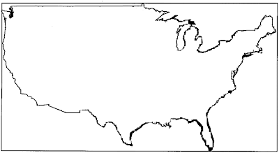
We started with a blank outline map of the U.S.


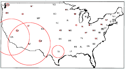
We finished with a map indicating the occurrences of coccidioidomycosis (as death certificate entries) in each state, and demonstrating the Southwest as an endemic area.


Each state has been "pasted" into the U.S. map. States with red circles contained cases of coccidioidomycosis recorded on death certificates; the diameter of circles is proportionate to the number of cases.

With a glance, we can see that coocidioidomycosis occurs primarily in the Southwest U.S. In fact, coccidioidomycosis, variously known as valley fever, San Joaquin Valley fever, California valley fever, and desert fever, is a fungal disease caused by Coccidioides immitis. In the U.S. this disease is endemic to certain parts of the Southwest.

The general method to make a data mashup map is as follows:

1. Find a map image, and determine the geographic boundaries of the map, in latitude and longitude.

In the case of the U.S. map, this is:

north border = 49 degrees latitude
south border = 25 degrees latitude
west border = 125 degrees longitude
east east = 66 degrees longitude

If we had geographic data on a smaller scale (e.g., a state, or a county, or a road or a river or a mountain range) we could have used a smaller map and all we'd need to change were the boundary values. The algorithm would be identical.

In general, the smaller the map the better. The reason for this is that the algorithm, as developed for our Perl script, needs a rectangular coordinate system. In large areas of the earth, surface curvature makes this difficult. When you project latitude-longitude points onto large area maps, using a simple proportionate scale, you can get some strange results. This is not a problem for maps that cover a small surface (i.e. a few hundred miles).

For yesterday's script, I used an outline map from the National Oceanic and Atmospheric Administration at:

http://www.nssl.noaa.gov/papers/techmemos/NWS-SR-193/images/fig7.gif

This image comes very close to being a recilinear map of the U.S.

2. The Ruby script requires the RMagick gem, the Ruby interface to the open source ImageMagick application.

Instructions for acquiring and installing RMagick are available from my web page:

http://www.julesberman.info/rubyhome.htm

Perl and Python also have interfaces to image methods, but I happen to find RMagick to be particularly easy to install and implement.

2. The Ruby script determines the boundaries of the map image, in pixels.

This is done with the imgage.columns method (to determine the width of the image in pixels) and the image.rows method (to determine the height of the image, in pixels).

3. All locations on the map can be determined by finding the proportionate number of pixels that account for the x,y distance (in latitude and longitude), and works from a list of the average latitude/longitude pairs for all of the continental states, plus the District of Columbia.

A list is available at:

http://www.maxmind.com/app/state_latlon

4. For each of the states, the Ruby script draws a circle, from the average latitude and logitude of the state, with a radius proportional to the number of cases of coccidioidomycoss reported in the CDC death certificate file, and prints the two-letter abbreviation for the state, a few pixels offsent from the circle's center.

lathash.each do
|key,value|
state = key
latitude = value.to_f
longitude = lonhash[key].to_f
l_y = (((north - latitude) / (north - south)) * height).ceil
l_x = (((west - longitude) / (west - east)) * width).ceil
gc.fill_opacity(0)
gc.stroke('red').stroke_width(1)
circlesize = ((sizehash[state].to_f)*2).to_i
gc.circle(l_x, l_y, (l_x - circlesize), l_y)
gc.fill('black')
gc.stroke('transparent')
gc.text((l_x - 5), (l_y + 5), state)
gc.draw(imgl)
end

If you want the script to display your finished image, you'll also need to include a widget module (I used Tk).

That's all there is to it. It takes a short while to get your supplementary files together and to install your required modules (if you don't already have these incredibly useful resources). The scripts are a few dozen lines in length, and many mashup projects can be done by simply tweaking these prototypical scripts. You can mashup disease data with anatomic images, or with cytogenetic images (chromosome maps), or with any image that relates a location to some quantitative data. The process is all basically the same.

In another blog for this series, we'll look at an example project where the raw data results may actually be more informative than the graphic visualization, and we'll discuss options for conveying undramatic data.

As I remind readers in almost every blog post, if you want to do your own creative data mining, you will need to learn a little about computer programming.

For Perl and Ruby programmers, methods and scripts for using a wide range of publicly available biomedical databases, are described in detail in my prior books:

Perl Programming for Medicine and Biology

Ruby Programming for Medicine and Biology

An overview of the many uses of biomedical information is available in my book,
Biomedical Informatics.

More information on cancer is available in my recently published book, Neoplasms: Principles of Development and Diversity.

In June, 2014, my book, entitled Rare Diseases and Orphan Drugs: Keys to Understanding and Treating the Common Diseases was published by Elsevier. The book builds the argument that our best chance of curing the common diseases will come from studying and curing the rare diseases.


I urge you to read more about my book. There's a generous preview of the book at the Google Books site. If you like the book, please request your librarian to purchase a copy of this book for your library or reading room.
© 2008 Jules Berman

As with all of my scripts, lists, web sites, and blog entries, the following disclaimer applies. This material is provided by its creator, Jules J. Berman, "as is", without warranty of any kind, expressed or implied, including but not limited to the warranties of merchantability, fitness for a particular purpose and noninfringement. in no event shall the author or copyright holder be liable for any claim, damages or other liability, whether in an action of contract, tort or otherwise, arising from, out of or in connection with the material or the use or other dealings.

tags: common disease, orphan disease, orphan drugs, rare disease, subsets of disease, disease genetics, genetics of complex disease, genetics of common diseases, ruby, perl, python, programming language, object-oriented programming, epidemiology, medical informatics

Wednesday, December 17, 2008

CDC Mortality Data: 8

This is the eighth in a series of posts on the CDC's (Centers for Disease Control and Prevention) public use mortality data sets. In a prior blog of this series, we discussed one of the earliest medical mashups, Dr. John Snow's map of cholera occurrences for the 1854 London epidemic..

Today, we'll show how we can use the CDC mortality data set to create a mashup, using short scripts written in Perl and Ruby. Readers of this blog who are specifically interested in the topic of Ruby-based mashups should also read Data Visualization with Ruby and RMagick - Where Are Those Bikes?, by LoGeek. LoGeek's elegant blog goes much further than mine to show how Ruby mashups can work with web service APIs.

Let's pretend that we know nothing about the geographic distribution of coccidioidomycosis (commonly misspelled coccidiomycosis). We can write a short Perl script that parses through every record in the CDC mortality file, pulling each death for which the diagnosis of coccidioidomycosis was recorded, and tallying the the deaths for the states in which the deceased death certificate was recorded. This will tell us something about the state-by-state distribution of coccidioidomycosis.

Here is a Perl script that produces a list of states and the tally of coccidioidomycosis cases, culled from the 1999 U.S. mortality file.

#/usr/local/bin/perl
open (STATE, "cdc_states.txt");
$line = " ";
while ($line ne "")
{
$line = <STATE>;
$line =~ /^[0-9]{2}/;
$state_code = $&;
$line =~ / +([A-Z]{2}) *$/;
$state_abb = $1;
$statehash{$state_code} = $state_abb;
}
close STATE;
open (ICD, "Mort99us.dat");
$line = " ";
while ($line ne "")
{
$line = <ICD>;
$state = 0;
$codesection = substr($line,161,140);
if ($codesection =~ /B38/)
{
$code = substr($line,20,2);
$state = $statehash{$code};
$state_tally{$state}++;
}
}
open (MAP, ">state_count.txt");
while ((my $key, my $value) = each(%state_tally))
{
print "$key $value\n";
print MAP "$key $value\n";
}
exit

The output of the Perl script looks like this:

AZ 62
CA 53
ID 2
IL 2
IN 1
KS 1
KY 1
MN 1
MO 1
MT 1
NC 2
NM 3
NV 3
NY 1
OH 1
OR 2
PA 1
TX 18
UT 2
WA 4
WI 2
WV 1

You'll notice that fewer than 50 states are included in the list. States that had no cases of coccidioidomycosis were not added to the list. We will see that this does not effect the mashup.

How did the Perl script compile the occurrences of coccidioidomycosis in from the CDC mortality files?

The CDC mortality files include the state of record for the death certificate in bytes 21 and 22 of the record. Each state is provided with a unique two digit code. The codes, and their corresponding state name, are provided in the CDC data dictionary for the mortality file. I simply prepared a text file, cdc_states.txt, that listed all the 2-digit codes and the corresponding state abbreviations, so the raw CDC data could be converted to universally recognizable abbreviations.

The script parses through each record, and pulls the 140-byte section of the record that contains the ICD disease codes corresponding to the conditions registered in the death certificate. In the ICD, coccidioidomycosis matches "B38". The Perl script finds all of the records that match "B38" and increases the appropriate state (from byte 21 and 22) tally by one. After the entire file is parsed, it prints out the list of states that have cases of coccidioidomycosis, along with their tallies.

Once that's done, we can mashup the disease data into a map of the United States. I found a public domain outline map of the U.S. on the National Oceanographic and Atmospheric Associationon web site. I "erased" the interior of the map, leaving a minimalist outline of the U.S. upon which to project the state-specific data. You can use any map, so long as you know the longitude and latitude boundaries.


A Ruby script inserts the state data onto the U.S. map.

#!/usr/local/bin/ruby -w
require 'RMagick'
north = 49.to_f #degrees latitude
south = 25.to_f #degrees latitude
west = 125.to_f #degrees longitude
east = 66.to_f #degrees longitude
#corresponds to the us continental extremities
text = File.open("c\:\\ftp\\loc_states.txt", "r")
lathash = Hash.new
lonhash = Hash.new
text.each do
|line|
line =~ /^([A-Z]{2})\,([0-9\.]+)\,\-?([\.0-9]+) *$/
state = $1
latitude = $2
longitude = $3
lathash[state] = latitude.to_f
lonhash[state] = longitude.to_f
end
text.close
text = File.open("c\:\\ftp\\state_count.txt", "r")
sizehash = Hash.new
text.each do
|line|
line =~ / /
state_abb = $`
state_value = $'
sizehash[state_abb] = state_value
end
text.close
imgl = Magick::ImageList.new("c\:\\ftp\\us\.gif")
width = imgl.columns
height = imgl.rows
gc = Magick::Draw.new
lathash.each do
|key,value|
state = key
latitude = value.to_f
longitude = lonhash[key].to_f
l_y = (((north - latitude) / (north - south)) * height).ceil
l_x = (((west - longitude) / (west - east)) * width).ceil
gc.fill_opacity(0)
gc.stroke('red').stroke_width(1)
circlesize = ((sizehash[state].to_f)*2).to_i
gc.circle(l_x, l_y, (l_x - circlesize), l_y)
gc.fill('black')
gc.stroke('transparent')
gc.text((l_x - 5), (l_y + 5), state)
gc.draw(imgl)
end
imgl.border!(1,1, 'lightcyan2')
imgl.write("circle.gif")
require 'tk'
root = TkRoot.new {title "view"}
TkButton.new(root) do
image TkPhotoImage.new{file "circle.gif"}
command {exit}
pack
end
Tk.mainloop
exit

Here is the result.


Each state has been "pasted" into the U.S. map. States with red circles contained cases of coccidioidomycosis recorded on death certificates; the diameter of circles is proportionate to the number of cases.

With a glance, we can see that coocidiomycosis occurs primarily in the Southwest U.S. In fact, coccidioidomycosis, variously known as valley fever, San Joaquin Valley fever, California valley fever, and desert fever, is a fungal disease caused by Coccidioides immitis. In the U.S. this disease is endemic to certain parts of the Southwest.

This post has gotten lengthy. In the next blog post of the CDC mortality series, I'll explain how the Ruby mashup script works.

© 2008 Jules Berman

As with all of my scripts, lists, web sites, and blog entries, the following disclaimer applies. This material is provided by its creator, Jules J. Berman, "as is", without warranty of any kind, expressed or implied, including but not limited to the warranties of merchantability, fitness for a particular purpose and noninfringement. in no event shall the author or copyright holder be liable for any claim, damages or other liability, whether in an action of contract, tort or otherwise, arising from, out of or in connection with the material or the use or other dealings.


Image of C. immitis in sputum sample.

Some additional information on Coccidioidomycosis is available from my web site.

In June, 2014, my book, entitled Rare Diseases and Orphan Drugs: Keys to Understanding and Treating the Common Diseases was published by Elsevier. The book builds the argument that our best chance of curing the common diseases will come from studying and curing the rare diseases.


I urge you to read more about my book. There's a generous preview of the book at the Google Books site. If you like the book, please request your librarian to purchase a copy of this book for your library or reading room.

tags: epidemiology, neoplasms, Ruby programming, rare diseases, genetic diseases, orphan diseases, complex diseases, orphan drugs, cdc, death certificates, mortality data

Tuesday, December 16, 2008

Ruby Programming for Medicine and Biology

As regular readers of this blog know, I am a free-lance science writer. I follow the sales of my books on Amazon.com. When Amazon deeply discounts my books, the sales go up. When they take the discounts off, sales drop precipitously. Because my books are geared to an elite audience (the same small group of people who read this blog), the books are all rather expensive (about $70-$75).

This morning, I noticed that Amazon just put a deep discount on my Ruby book (Ruby Programming for Medicine Biology). It's now $43.50 (a 36% discount from full price). So if there are any blog readers who have been reluctant to buy at the regular price, there's a price break in effect currently.

-Jules Berman

Monday, December 15, 2008

CDC Mortality Data: 7

This is the seventh in a series of posts on the CDC's (Centers for Disease Control and Prevention) public use mortality data sets. Yesterday, we introduced the concept of data mashups. The next several blogs will describe mashup techniques. For today's blog, let's focus on the kinds of biological questions that can be approached with the CDC data. You can't design a credible mashup until you've acquired some understanding of the potential value of the mashed up data.

Alpha-1 antitrypsin disease is a prototypical serpinase disease (disease due to deficiencies or abnormalities in the synthesis of serine proteinases). People with this disorder are homozygous for mutations in the alpha-1 antitrypsin gene. The full-blown disease is characterized by cirrhosis and emphysema. The pathogenesis of this diseases is somewhat complex, because there are a variety of different possible mutations of the gene, and the clinical manifestations vary somewhat with the mutation type. The cirrhosis is apparantly due to the intracellular accumulation of abnormal alpha-1 antitrypsin molecules within hepatocytes, and the emphysema is apparently the result of destructive effects of inflammation-induced intrapulmonary trypsin levels, unopposed by antitrypsin.

As is the case in most rare recessive genetic disorders, heterozygous mutations in the alpha-1 antitrypsin gene are found as common gene variants in the general population.

If a double-dose (homozygous) of an altered gene causes disease, what is the effect of a single (heterozygous) gene variant? Gene variations may be responsible for differences in the pathogenesis of disease among members of the apparently healthy public. About 15% of smokers develop COPD (chronic obstructive pulmonary disease) or emphysema. Why does one smoker develop COPD, while another smoker escapes pulmonary toxicity? Might the difference be accounted for by gene variations, and might a key gene be the alpha-1 antitrypsin gene?

A number of researchers have provided data indicating that heterozygous carriers of alpha-1 antitrypsin mutations are at increased risk for developing emphysema (Lieberman 1969 and Stevens 1971).

Lieberman, J.: Heterozygous and homozygous alpha-1-antitrypsin deficiency in patients with pulmonary emphysema. New Eng. J. Med. 281: 279-284, 1969.

Stevens, P. M.; Hnilica, V.; Johnson, P. C.; Bell, R. L.: Pathophysiology of hereditary emphysema. Ann. Intern. Med. 74: 672-680, 1971.

Population studies indicate that the African American population has much lower levels of alpha-1 antitrypsin disease gene variants than whites, the most prevalent mutations occurring in people with European ancestry (DeCroo 1991, Hutchison 1998).

DeCroo, S.; Kamboh, M. I.; Ferrell, R. E.:Population genetics of alpha-1-antitrypsin polymorphism in US whites, US blacks and African blacks. Hum. Hered. 41: 215-221, 1991.

Hutchison, D. C. S.: Alpha-1-antitrypsin deficiency in Europe: geographical distribution of Pi types S and Z. Resp. Med. 92: 367-377, 1998.

We hypothesize that if alpha-1 antitrypsin disease mutations plays a significant contributory role role in the pathogenesis of emphysema in the general population, we can expect to see fewer emphysema cases in African-Americans (who are unlikely to be heterozygous for alpha-1 antitrypsin diseases mutations) than the white population. We can test this hypothesis by determining the percentage of African-Americans who die, in the U.S., with emphysema, and comparing that number with the percentage of White Americans who die with emphysema.

Here's the Perl script:

#/usr/local/bin/perl
open (ICD, "Mort99us.dat");
$line = " ";
while ($line ne "")
{
$line = <ICD>;
$count++;
$codesection = substr($line,161,140);
$race = substr($line,59,2);
$whitecount++ if ($race eq "01");
$blackcount++ if ($race eq "02");
if ($codesection =~ /J4[34]/)
{
$whiteemp++ if ($race eq "01");
$blackemp++ if ($race eq "02");
}
}
close ICD;
$whiteempfrac = 100 * ($whiteemp / $whitecount);
$blackempfrac = 100 * ($blackemp / $blackcount);
print "Total records in file is $count\n";
print "Total African-Americans in file is $blackcount\n";
print "Total Whites in file is $whitecount\n";
print "Total African-Americans with emphysema $blackemp\n";
print "Total Whites with emphysema is $whiteemp\n";
print "Percent African-Americans with emphysema is ";
print substr($blackempfrac,0,4) . "\n";
print "Percent Whites with emphysema is ";
print substr($whiteempfrac,0,4) . "\n";
exit;

Here is the output from the script:

Total records in file is 2394872
Total African-Americans in file is 285276
Total Whites in file is 2064169
Total African-Americans with emphysema 15190
Total Whites with emphysema is 222996
Percent African-Americans with emphysema is 5.32
Percent Whites with emphysema is 10.8

The Perl script parses through the CDC mortality data for 1999.

Race is assigned a two digit code, 01 for White and 02 for Black, at bytes 60 and 61 of each record. The race code is pulled with the Perl statement:

$race = substr($line,59,2);

Emphysema and COPD cover ICD codes that begin with J4, followed by 3 or 4. Cases coded or emphysema or COPD are matched with the following Perl condition:

if ($codesection =~ /J4[34]/)

The Perl script examines 2.3 million death records in the CDC data set, informs us that African Americans have about half the rate of emphysema and COPD as does the White population. This observation is consistent with our hypothesis that the alpha-1 antitrypsin gene variant increases the risk of emphysema in the general population.

Does this observation prove the hypotheses? Absolutely not. The same observation could be explained by many different hypotheses. But we have shown, with a large number of cases (nearly a quarter million emphysema/COPD cases), that African-Americans have less disease than Whites.

This is the kind of analysis that uses existing CDC mortality data sets to develop and test a hypothesis. In the next few blogs, as we start to use CDC data in mashup applications, we will be developing hypotheses that relate our available data with informaiton that has a graphic representation (such as a map, or a physical drawing of a chromosome, or an anatomic picture).

© 2008 Jules Berman

As with all of my scripts, lists, web sites, and blog entries, the following disclaimer applies. This material is provided by its creator, Jules J. Berman, "as is", without warranty of any kind, expressed or implied, including but not limited to the warranties of merchantability, fitness for a particular purpose and noninfringement. in no event shall the author or copyright holder be liable for any claim, damages or other liability, whether in an action of contract, tort or otherwise, arising from, out of or in connection with the material or the use or other dealings.
In June, 2014, my book, entitled Rare Diseases and Orphan Drugs: Keys to Understanding and Treating the Common Diseases was published by Elsevier. The book builds the argument that our best chance of curing the common diseases will come from studying and curing the rare diseases.


I urge you to read more about my book. There's a generous preview of the book at the Google Books site. If you like the book, please request your librarian to purchase a copy of this book for your library or reading room.

tags: common disease, orphan disease, orphan drugs, rare disease, subsets of disease, disease genetics, genetics of complex disease, genetics of common diseases, cryptic disease, cdc, epidemiology, neoplasms

CDC Mortality Data: 6

This is the sixth in a series of posts on the CDC's (Centers for Disease Control and Prevention) public use mortality data sets.

Yesterday, we showed how to create a dictionary of ICD code/term pairs that could be used to assign disease terms to the death certificate record codes occurring in the CDC Mortality data sets. This morning I prepared a , web page that contains output data, from yesterday's blog post, that could not fit in the blog page.

I also mentioned, yesterday, that I would explain how the CDC data could be used in mashup projects. So, today, we'll begin a series of blogs that explain how mashup technology can integrate the CDC mortality data sets, and answer biomedical hypotheses.

Data mashups combine and integrate different data sources to produce a graphical representation of data that could not be achieved with any single available data source. Many people apply the term "mashup" to Web-based applications that employ two or more web services or that use two or more web-based applications that have web-accessible APIs (Application Progam Interfaces) that permit their data to be integrated into a derivative application. Because I am a biomedical information specialist, I apply "mashup" to any application that integrates available biomedical data sources, to answer questions with a graphic output (with or without Web involvement).

The classic medical mashup was done by Dr. John Snow, in London, in 1854. Wikimedia has an excellent essay on the subject. The story goes that a major outbreak of cholera occurred in late-August and early September of 1854, in the Soho district of London. By the end of the outbreak, 616 people died.

At the time, nobody understood the biological cause of cholera. At the height of the outbreak, Dr. Snow conducted a rapid, interview-based survey of the site of occurrences of new cases of cholera, producing a case-density map (hand-drawn by the doctor himself).


This map is now in the public domain. A higher-resolution version of the map is available from Wikimedia.

Examination of the map revealed that the epidemic expanded from a water source, the Broad Street pump. The pump was quickly shut. Dr. Snow's historic mashup is sometimes credited with ending the cholera epidemic and heralding a new age in scientific biomedical investigation.

To create a map mashup, we will need a data source that lists occurrences of disease and the localities in which they occur; a data source that provides the latitude and longitude of localities, and a map whose East, West, North, and South boundaries have known latitudes and longitudes. We will also need a programming language that can transform data to graphics and transfer graphics to a a map. We'll use Ruby because I like the Ruby interface to Image Magick, but Perl or Python would work equally well.

Much more importantly, we will need to have a question or hypothesis, whose solution requires a mashup. Much of computational medicine can be described as a solution in search of a question. We have many ways of analyzing data, but we often lack important questions. In the next several blogs, we will show how the CDC mortality data files can be used to test medical hypotheses. Through examples, we will introduce concepts and tools used in mashups, and we will end this series with several mashups, of increasing complexity.

If you are new to this blog, you might want to review the prior 5 blog posts, in the series, sequentially.

As I remind readers in almost every blog post, if you want to do your own creative data mining, you will need to learn a little about computer programming.

For Perl and Ruby programmers, methods and scripts for using a wide range of publicly available biomedical databases, are described in detail in my prior books:

Perl Programming for Medicine and Biology

Ruby Programming for Medicine and Biology

An overview of the many uses of biomedical information is available in my book,
Biomedical Informatics.

More information on cancer is available in my recently published book, Neoplasms: Principles of Development and Diversity.

© 2008 Jules Berman

As with all of my scripts, lists, web sites, and blog entries, the following disclaimer applies. This material is provided by its creator, Jules J. Berman, "as is", without warranty of any kind, expressed or implied, including but not limited to the warranties of merchantability, fitness for a particular purpose and noninfringement. in no event shall the author or copyright holder be liable for any claim, damages or other liability, whether in an action of contract, tort or otherwise, arising from, out of or in connection with the material or the use or other dealings in the material.

Sunday, December 14, 2008

CDC Mortality Data: 5

This is the fifth in a series of posts on the CDC's (Centers for Disease Control and Prevention) public use mortality data sets.

In the fourth blog of this series, we learned how the cause of death data from death certificate records is is transformed into a mortality record consisting of an alphanumeric sequence. The causes of death are represented by ICD codes. If we have a computer computer-parsable list of ICD codes, we can write a short program that assigns human-readable terms (full names of diseases) to the codes in the mortality files.

Let's start with the each10.txt file, available by anonymous ftp from the ftp.cdc.gov web server at:

/pub/Health_Statistics/NCHS/Publications/ICD10/each10.txt

Here are the first few lines of this file:

A00Cholera
A00.0Cholera due to Vibrio cholerae 01, biovar cholerae
A00.1Cholera due to Vibrio cholerae 01, biovar el tor
A00.9Cholera, unspecified
A01Typhoid and paratyphoid fevers
A01.0Typhoid fever
A01.1Paratyphoid fever A
A01.2Paratyphoid fever B
A01.3Paratyphoid fever C
A01.4Paratyphoid fever, unspecified
A02Other salmonella infections
A02.0Salmonella gastroenteritis

There are 9,320 terms in the each10.txt file, sufficient for many purposes. However, the entries in each10.txt were selected from a much larger collection of ICD10 terms. The terms in the each10.txt file are "cause of death" concepts. They will match causes of death found on Death Certificates. However, Death Certificates (and hence the public use CDC mortality data sets) include "other significant conditions" in addition to causes of death (discussed in yesterday's blog). If we want to find the meaning of all of the conditions contained in the CDC mortality files, we need to supplement the each10.txt file with additional ICD10 entries.

More ICD10 entries are found in the i10idx0707.pdf file, a large index of ICD10 terms and their codes. This file is also available by anonymous ftp from the CDC server at:

ftp.cdc.gov
/pub/Health_Statistics/NCHS/Publications/ICD10CM/2007/i10idx0707.zip

Download and unzip this file (a freeware unzip utility is available at http://www.7zip.com/)

The unzipped file is an Adobe Acrobat pdf file 1,344 pages in length. An excerpt from the first page of the .pdf file is shown:


We need to convert this .pdf file into a .txt fie, if we expect to parse through the file and extract codes and matching terms. For most .pdf files, you can simply select, cut, and paste pages into a .txt file. This is a tricky method to use for very large files, because it requires a lot of memory. Sometimes the textual output from .pdf files is garbled or contains errors. Some .pdf files do not support cut and paste operations.

I like to convert .pdf files to .txt files in a two-step operation using free, open source command-line pdf utilities: pdftk and xpdf.

pdftk is available at: http://www.accesspdf.com/pdftk/
The zipped .exe file is pdftk-1.12.exe.zip

xpdf is available at: http://www.foolabs.com/xpdf/download.html
The zipped .exe file is xpdf-3.02pl2-win32.zip

Many .pdf files come in an internally compressed format. The compression is not apparent to the user. There is no special file extension, and the Adobe Reader software decompresses the file seamlessly. Before converting compressed .pdf files to text, we need to decompress the file.

From the command line in pdftk subdirectory, uncompress the compressed .pdf file with the following command. Remember to copy the i10idx0707.pdf file to the pdftk subdirectory.

C:\pdftk>pdftk i10idx0707.pdf output mydoc_un.pdf uncompress

Now we have an uncompressed .pdf file, mydoc_un.pdf

From the xpdf subdirectory, we can convert the uncompressed pdf file to a .txt file. Remember to copy the mydoc_un.pdf file to the pdftk subdirectory.

C:\xpdf>pdftotext mydoc_un.pdf mydoc.txt

This produces a text (ASCII) version of the icd10 index file:

MYDOC.TXT (2,360,138 bytes)

At last, we have two .txt files (mydoc.txt and each10.txt) that we can use, together, to create a clean, computer-parsable list of ICD codes and their equivalent terms, in English.

Here is the Perl script that does the job. You will need to place the mydoc.txt file and the each10.txt file in the same subdirectory as the Perl script.

#!/usr/bin/perl
open(TEXT, "mydoc.txt");
undef($/);
$var = <TEXT>;
close TEXT;
$var =~ tr/\14//d;
$var =~ s/ ([A-Z][0-9][0-9\.]*[0-9])/ $1\n/g;
open(TEXT, ">mydoc.out");
print TEXT $var;
close TEXT;
$/ = "\n";
open(TEXT, "mydoc.out");
$line = " ";
while ($line ne "")
{
$line = <TEXT>;
if ($line =~ /\b([A-Z][0-9][0-9\.]*[0-9]) *$/)
{
$term = $`;
$code = $1;
$term =~ s/^[ \-]*//o;
$term =~ s/[ \-]*$//o;
$term = lc($term);
$line =~ tr/\173//d;
$dictionary{$code} = $term;
}
}
close TEXT;
open (ICD, "each10.txt")||die"cannot";
undef($/);
$line = <ICD>;
$line =~ tr/\000-\011//d;
$line =~ tr/\013-\014//d;
$line =~ tr/\016-\037//d;
$line =~ tr/\041-\055//d;
$line =~ tr/\173-\377//d;
@linearray = split(/\n(?=[ ]*[A-Z][0-9\.]{1,5})/, $line);
foreach $thing (@linearray)
{
if ($thing =~ /^ *([A-Z][0-9\.]{1,5}) ?/)
{
$code = $1;
$term = $';
$term =~ s/\n//;
$term =~ s/[ ]+$//;
$dictionary{$code} = $term;
}
}
unlink("mydoc.out");
open (TEXT, ">mydoc.out");
foreach $key (sort keys %dictionary)
{
print TEXT "$key $dictionary{$key}\n";
}
close TEXT;
exit;

The output file is: mydoc.out (1,091,342 bytes). It contains about 23,000 code/term pairs

I renamed the mydoc.out file, icd10_pl.txt. We will use this file in the next Perl script, to determine the total number of each condition appearing in the 1+ Gbyte mort99us.dat file. You will need to placed the icd10_pl.txt file and the Mort99us.dat file in the same subdirectory as this Perl script.

#/usr/local/bin/perl
open (ICD, "icd10_pl.txt");
$line = " ";
while ($line ne "")
{
$line = <ICD>;
if ($line =~ /^([A-Z][0-9\.]+) +/)
{
$code = $1;
$term = $';
$code =~ s/\.//o;
$term =~ s/\n//;
$term =~ s/ +$//;
$dictionary{$code} = $term;
}
}
close ICD;
open (ICD, "Mort99us.dat");
$line = " ";
print "\n\n";
while ($line ne "")
{
$line = <ICD>;
$codesection = substr($line,161,140);
@codearray = split(/ +/,$codesection);
foreach $code (@codearray)
{
$code =~ /[A-Z][0-9]+/;
$code = $&;
$counter{$code}++;
}
}
close ICD;
open (OUT, ">cdc.out");
while ((my $key, my $value) = each(%counter))
{
$value = "000000" . $value;
$value = substr($value,-6,6);
push(@filearray, "$value $key $dictionary{$key}");
}
$outfile = join("\n", reverse(sort(@filearray)));
print OUT $outfile;
exit

On my 2.5 GHz CPU desktop computer, it takes well under a minute to parse through the 1+ Gbyte CDC mortality data set and produce the desired output file (cdc.out). The total number of records parsed by the script were 2394871. There are 5,650 conditions included in the 1999 CDC mortality data set.

The first 45 lines of the output file are:

412827 I251 Atherosclerotic heart disease
352559 I469 Cardiac arrest unspecified
273644 I500 Congestive heart failure
244162 I219 Acute myocardial infarction unspecified
210394 J449 Chronic obstructive pulmonary disease unspecified
206996 J189 Pneumonia unspecified
203906 I10 Essential primary hypertension
176834 I64 Stroke not specified as hemorrhage or infarction
162128 C349 Bronchus or lung unspecified
149777 E149 Without complications
143326 J969 Respiratory failure unspecified
129947 A419 Septicemia unspecified
115504 F03 Unspecified dementia
106137 N19 Unspecified renal failure
101224 I250 Atherosclerotic cardiovascular disease so described
075834 G309 Alzheimers disease unspecified
073365 I709 Generalized and unspecified atherosclerosis
072931 R092 Respiratory arrest
067525 I499 Cardiac arrhythmia unspecified
067055 I48 Atrial fibrillation and flutter
065657 C80 Malignant neoplasm without specification of site
056718 J690 Pneumonitis due to food and vomit
056425 C189 Colon unspecified
051698 C509 Breast unspecified
045707 C61 Malignant neoplasm of prostate
043191 I429 Cardiomyopathy unspecified
038127 N189 Chronic renal failure unspecified
038072 E119 Without complications
037810 I119 Hypertensive heart disease without congestive heart failure
036801 I739 Peripheral vascular disease unspecified
036151 D649 Anemia unspecified
035720 N390 Urinary tract infection site not specified
035552 K922 Gastrointestinal hemorrhage unspecified
035133 J439 Emphysema unspecified
031981 K746 Other and unspecified cirrhosis of liver
031327 E86 Volume depletion
031266 G20 Parkinsons disease
031050 N180 Endstage renal disease
030693 N179 Acute renal failure unspecified
030442 R99 Other illdefined and unspecified causes of mortality
030416 C259 Pancreas unspecified
030248 K729 Hepatic failure unspecified
028458 I255 Ischemic cardiomyopathy
026860 I269 Pulmonary embolism without mention of acute cor pulmonale
026445 I509 Heart failure unspecified

The top line is:

412827 I251 Atherosclerotic heart disease

It indicates that atherosclerotic heart disease is the most common condition listed in the death certificates in 1999 in the U.S. It was listed 412,827 times. The ICD10 code for Atherosclerotic heart disease is I25.1.

Some of the output lines do not seem particularly helpful. For example:

056425 C189 Colon unspecified
051698 C509 Breast unspecified

Nobody dies from "Colon unspecified." The strange diagnosis is explained by the rather unsatisfactory way that the ICD assigns terms to codes. In this case, "Colon unspecified" is a sub-term in the general category of "Neoplasms of the colon." We know this because all of the codes beginning with "C" (i.e., C189 and C509 in this case) are cancer codes. Whenever an ICD term appears un-informative, we can return to the ICD10_pl.txt file (created in yesterday's blog) and clarify its meaning by examining the root term for the sub-term.

In the next blog in this series, we will try a more ambitious project, using the CDC mortality data and the U.S. map in a Ruby mashup script.

As I remind readers in almost every blog post, if you want to do your own creative data mining, you will need to learn a little computer programming.

For Perl and Ruby programmers, methods and scripts for using a wide range of publicly available biomedical databases, are described in detail in my prior books:

Perl Programming for Medicine and Biology

Ruby Programming for Medicine and Biology

An overview of the many uses of biomedical information is available in my book,
Biomedical Informatics.

More information on cancer is available in my recently published book, Neoplasms.

© 2008 Jules Berman

As with all of my scripts, lists, web sites, and blog entries, the following disclaimer applies. This material is provided by its creator, Jules J. Berman, "as is", without warranty of any kind, expressed or implied, including but not limited to the warranties of merchantability, fitness for a particular purpose and noninfringement. in no event shall the author or copyright holder be liable for any claim, damages or other liability, whether in an action of contract, tort or otherwise, arising from, out of or in connection with the material or the use or other dealings in the material.


My book, Principles of Big Data: Preparing, Sharing, and Analyzing Complex Information was published in 2013 by Morgan Kaufmann.


I urge you to explore my book. Google books has prepared a generous preview of the book contents.

tags: big data, metadata, data preparation, data analytics, data repurposing, datamining, data mining, neoplasms, nomeclature, Perl script